Salary Prediction
Introduction to Application:
Nowadays, the wage of an employee is a major factor in deciding whether or not to stay with a company. Employees are constantly changing companies in order to obtain the desired results. An employer's duty of predicting a reasonable salary for an employee is always difficult. In this blog, we provide a salary prediction model with an appropriate algorithm that uses essential features to forecast an employee's wage.
We are glad to share with you the standard code which you could use on our CODER to execute on the same dataset or your own dataset to build your own model.
Objectives of the Model:
Building a predictive algorithm to predict the salary of an employee given how many years of experience they have.
Principle:
This is a Data Science model where the machine learning learns from the categorical and continuous variables in the form of historical data which would in turn to used train the model better prediction and accuracy.
Introduction to Dataset:
The dataset used in the project is the Salary Dataset taken from the Kaggle website. It has 2 columns — “Years of Experience” and “Salary” for 30 employees.
Dataset Link:https://raw.githubusercontent.com/schoolforai/AI-Models/main/salaries.csv

Methodology - SFAI's 5 Stage Approach

As you may be aware, any AI application could fall into one of these five stages. You probably learned about them in your Level 2: Data Science class. From data sourcing to deployment, this strategy would make AI application development more understandable. Please note that all applications at SchoolforAI are broken down into these 5-stages for better control. These five stages would be followed by every machine learning engineer. However, it is not always possible or necessary to demonstrate a few steps. For example, only a few data sets may necessitate Data Preparation and Feature Engineering. As a result, these 5-stages may need to be condensed.
As the purpose of this application is to introduce how we build a Data Science model, we have excluded or merged few stages to finalize with the below steps:
1. Data Sourcing
Data sourcing is the primary stage of find the relevant data for the model. For this model we are using Online Salary Data from Kaggle. You could see the data in this stage and understand about its type, number of records, features and such. In the below code you would find the procedure to include all the required libraries and how to read the data form the location.
# Essential Libraries

import pandas as pd
import numpy as np
import matplotlib.pyplot as plt
import seaborn as sns
from sklearn.model_selection import train_test_split
from sklearn.linear_model import LinearRegression
from sklearn.metrics import r2_score,mean_squared_error, mean_absolute_error
import math
import joblib

#Data Reading
data = pd.read_csv(r"file path")
var = data.columns

# To get information
def info(data):
    print(data.info())

# Calling Function
info(data)

# To get shape of data
def shape(data):
    print(data.shape)
    # Calling Function
shape(data)
2. Model Building
In this step we have merged EDA & FE, Algo Selection and Optimization for simplicity purpose. EDA is a essential process where you try to explore the interdependencies in the data.
We must check for missing values and outliers before doing EDA. The code below demonstrates how to calculate the missing count and check for data outliers.
# Checking for missing values
def missingcount(data):
    return data.isnull().sum()

# To Detect Outliers

def outliers(data,var):
    num_vars=[var for var in data.columns if data[var].dtypes != 'O']
    for var in num_vars:
        images=data.boxplot(column=var) #
        plt.title(images)
        plt.show()

# Calling Function
images=outliers(data,var)
However, the provided dataset is cleaned, we will proceed with Data Visualization. Below is the code for Data Visualization.
# Data Visualization

                    # Categorical Data Visualization

# # Univariate Analysis

def uni_cat(data,var):
    cat_vars=[var for var in data.columns if len(data[var].unique())<20]
    for var in cat_vars:
        sns.countplot(x=data[var],data=data)
        plt.show()

uni_cat(data,var)

# # Bivariate Ananlysis

def bi_cat(data,var):
    cat_vars=[var for var in data.columns if len(data[var].unique())<20]
    for var in cat_vars:
        target=data['price'] # User Defined Variable
        sns.countplot(x=data[var],hue=target,data=data)
        plt.show()

bi_cat(data,var)

                 # Continuous Data Visualization

# # Univariate Analysis

def uni_cont(data,var):
    num_vars=[var for var in data.columns if data[var].dtypes != 'O']
    for var in num_vars:
        data[var].hist(bins=30)
        plt.show()
        plt.title(var)

uni_cont(data,var)

# # Bivariate Ananlysis

def bi_cont(data,var):
    num_vars=[var for var in data.columns if data[var].dtypes != 'O']
    for var in num_vars:
        target=data['price'] # User Defined Variable
        plt.scatter(data[var],salary)
        plt.show()
Feature engineering helps in working on the features and selecting the right features (columns) that would contribute to the models power of predictability. In this case we are retaining all the features.
You must have already understood from your classes that selection of algorithm depends on the type of output or label in the dataset, i.e. either categorical or continuous output. As the target value in our dataset is categorical data we have considered it as the classification problem.
For the given dataset, we have tried several algorithms to finalized on Simple Linear Regression that suits our classification problem. Below is the syntax for the Simple Linear Regression. It would help to understand each parameter and its effect on the final accuracy. However, for simplicity we have considered only few important parameters for turning purpose.
In our SchoolforAI app, you could change the parameters to tune the algorithm for the given dataset to achieve maximum possible accuracy. You can see that in the below image.
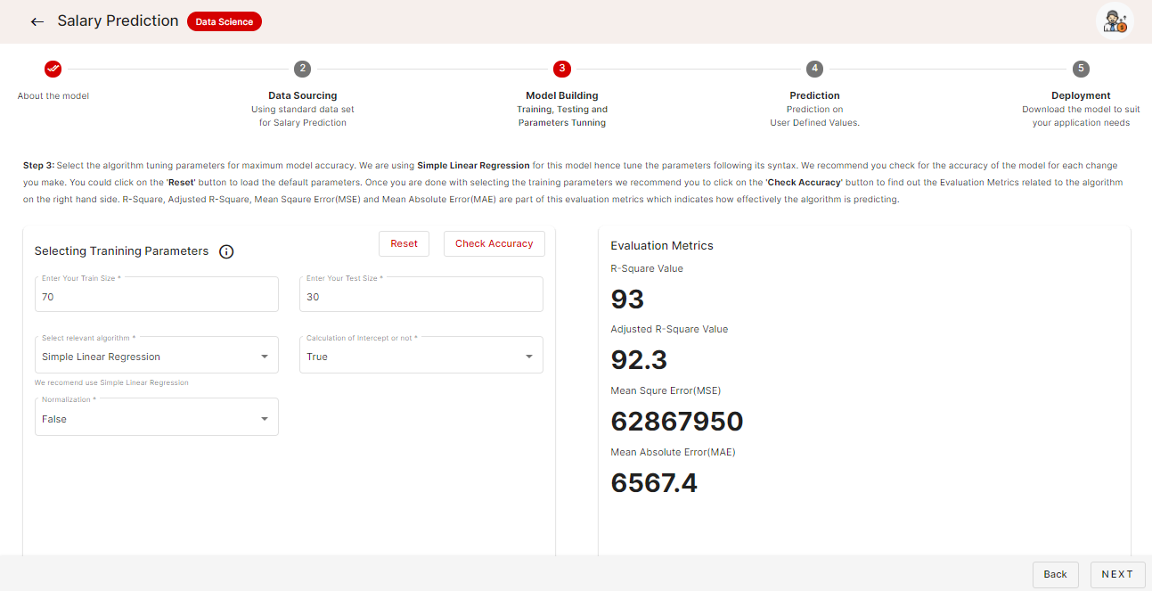
What you are doing here is finding the best possible parameters to train the model for highest possible accuracy. Once you are done with the tuning and training you could proceed to the next step. Please note down the final optimization parameters you have used for training the algorithm, for your reference.
# Dependent & Independent Variables Seperation

# Dependent Variable
def dependent(data):
    x=data.iloc[:,-1]
    return x

y=dependent(data)

# Independent Variable

def Independent(data):
    x=data.iloc[:,:-1]
    return x

X=Independent(data)
The code below is for Model Building. You can see how we implemented the model in the code.
# Data Splitting into training and testing

def train_test(X,y):
    X_train,X_test,y_train,y_test = train_test_split(X,y,train_size=0.8,random_state=0)

    return X_train,X_test,y_train,y_test

X_train,X_test,y_train,y_test = train_test(X,y)

# Model(LineraRegression) Building and Model Fitting

def modelfitting(x,y):
    lr=LinearRegression(fit_intercept=True,
                        normalize=False)
    lr.fit(x,y)
    joblib.dump(lr,'model_joblib') # Model Serilization
    print(lr.get_params())

modelfitting(X_train,y_train)
4. Data Validation
Once the training and parameter tuning is done it is time to cross check or validate the model with a new set of set. In this stage you would input a new set of data for the model to predict the output. This is the real-life scenario where the model we have built would be put to test.
You can see how we can predict the outcome from the test inputs in our SchoolforAI app in the image below.
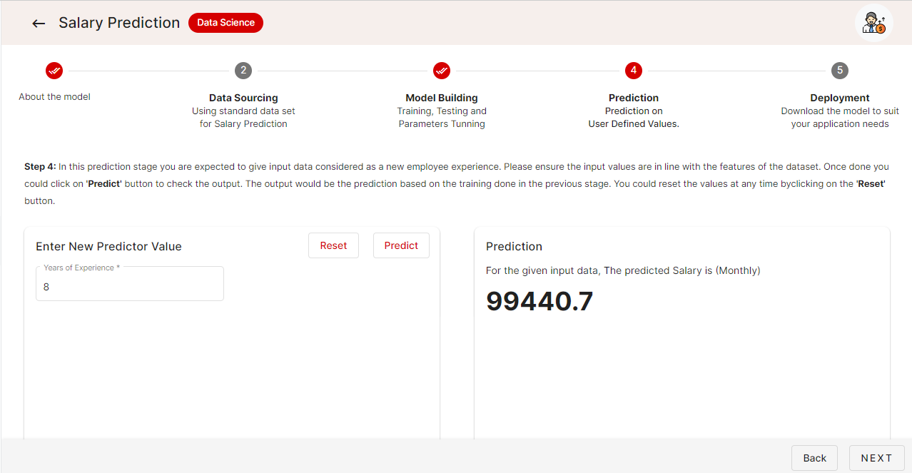
This is how you test a model.
# Data Validation
y_predict = []

def predict(z):
    model=joblib.load('model_joblib')
    model.predict(z)
    y_hat = model.predict(z)
    y_predict.append(y_hat)

    return y_predict
Below is the code for evaluating the model prediction.
# Checking R-Squre Value

def R_sqr(X, y):
    model=joblib.load('model_joblib')
    R_sqr = model.score(X, y)
    return R_sqr

# Mean Squared Error

def mse(y_test, y_predict):
    model=joblib.load('model_joblib')
    y_predict=model.predict(X_test)
    mse = mean_squared_error(y_test, y_predict)
    return mse

# Mean Absolute Error

def mae(y_test, y_predict):
    model=joblib.load('model_joblib')
    y_predict=model.predict(X_test)
    mse = mean_absolute_error(y_test, y_predict)
    return mse
5. Deployment
Once we are happy with the model, parameter tuning and the offered accuracy we would proceed with deployment. It could be on cloud or on customer’s server. This needs some additional skills such as FLASK. For the convenience and learning of the students the standard code could be downloaded in this stage. You could load the code into our CODER and practice.
Coder link: https://app.schoolforai.com/coder/python
Source: https://app.schoolforai.com/ai-coder/salary-prediction